Handling Concept Drift at the Edge of Sensor Networks

Consider a scenario where you're using an electric motor in your workshop. You've installed a few sensors on the outer body of this motor and these sensors continuously send you data over WiFi. Then you have an elaborate setup on the cloud where your intelligent application program analyses those parameters and determines the health status of your motor.

This, of course, takes into account the trained pattern of motor vibration and current consumption by the motor during the learning phase. And, so long nothing changes, this pattern recognition works like a charm. That's what a good machine learning would entail.

Image courtesy: abb.com

However, this data generated by an electric motor can change over time. This can result in poor analytical results, which otherwise have assumed a static relationship between various parameters and motor health.

The change in data can occur due to various real-life scenarios, such as changes in operating load conditions, aging of ball bearings or foundation on which the motor is installed, environmental conditions, etc.

This problem of change in data over time, thereby affecting statically programmed (or assumed) underlying relationships, is a common occurrence for several other real-life scenarios of machine learning. The technical term for this scenario in the field of machine learning is “concept drift”.

"A concept in "concept drift" refers to the unknown and hidden relationship between inputs and output variables. For example, one concept in weather data may be the season that's not explicitly specified in temperature data but may influence temperature data. Another example may be customer purchasing behavior over time that may be influenced by the strength of the economy, where the strength of the economy isn't explicitly specified in the data. These elements are also called a 'hidden context'."

— The Problem of Concept Drift: Definitions and Related Work.

Why Is This a Problem?

For a completely static Applications, concept drift isn't a problem at all. In several Applications, however, the relationship between input parameters (or features) and output characteristic change over time. If your machine learning model did assume data patterns to be static, then there will be a problem in the future.

It's still relatively easy to handle if these relationships and formulas are maintained on the cloud. You can easily update new relationship formulas in the cloud application and everything will be set.

However, if your architecture is edge compute dependent, like the models being pushed to the edge sensors for faster responses, then this (new) learning must be transferred. In the cases of industrial implementation, edge computing utilization is highly recommended and is quite common.

The challenge here is, how do you update these formulas in low-cost sensors that do not have a vast memory advantage or where the over the air firmware (OTA) updates are not feasible? How can you just send and update only the important formulas to that one sensor device?

Challenges in Dealing With Concept Drift

The first challenge is to detect when this drift occurs; here are two ways to handle that:

1. When a model is finalized for deployment, record its baseline performance parameters such as accuracy, skill level, etc. Then, when the model is deployed, periodically monitor these parameters for change. If you see a significant change in parameters, that could be indicative of potential concept drift and you should take action to fix it.
2. The other way to handle this is to assume that drift will occur and, therefore, periodically update the model, the sensors or edge network. The challenge, however, is to handle these updates in edge sensors without causing any downtime.

While the first challenge is relatively easy to manage, the second can be a difficult technical problem. This is where having a capability built-in to the sensors to be able to accept model updates without needing to update the entire firmware becomes important. This is where the dynamic evaluation algorithm would come in handy.

The Dynamic Evaluation Algorithm

The fundamental algorithm was first introduced in 1954 and was first used in desktop calculators by HP in 1963. Now, almost all the calculators deploy this methodology to perform calculations of user inputs.

The algorithm heavily relies on a specific type of representation of the formula that's known as Postfix Notation or Reverse Polish Notation (RPN).

In Postfix Notation the operators follow their operands; for instance, to add 4 and 6, one would write 4 6 + rather than 4 + 6. If there are multiple operations, the operator is given immediately after its second operand. The expression 1 – 4 + 6 written in conventional notation  would be written as 1 4 – 6 + in Postfix.

An advantage of Postfix is that it removes the need for parentheses that are required by normal notations and thus removes ambiguity from the formula. For instance, 1 – 4 * 6 can also be written 1 – (4 * 6) and it's quite different from (1 – 4) * 6. In Postfix, the former could be written 1 4 6 * –, which unambiguously means 1 (4 6 *) – whereas the latter could be written 1 4 – 6 * or 6 1 4 – *.

In either case, you would see that operators with a higher priority would come on far right. As the notation result is always context-free, once an equation is converted to Postfix Notation, it becomes easier for a computer to evaluate the same equation using an outside-in evaluation sequence.

Using Postfix in Sensors on the Edge

A typical method to convert normal formulas to Postfix Notation in software code has two steps — first, construct an abstract syntax tree and, second, perform a post-order traversal of that tree.

Once the notation is created it needs to be evaluated, and to carry out the outside-in evaluation sequence, we must use a stack. This means our processor must have sufficient stack (RAM) available. It's obvious that limited or small RAM availability would mean limited computation ability.

1. Tokenization

This algorithm is stack and queue dependent and uses a stack for storing functions (operators) and a simple queue to hold numbers (operands).

The figure below shows the algorithm flowchart. Due to the nature of operations performed in this algorithm, it's also called a Shunting Yard Algorithm since the operation resembles the railroad shunting yard methodology.

Shunting Yard algorithm

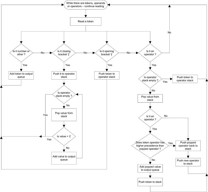
With this flow, a valid equation can be parsed into a tokenized sequence.

2. Evaluation

Once we finish the token parsing and formulate the appropriate notation sequence, the next step is the evaluation of an answer. It can be done in the following steps:

1. Initialize an empty stack.
2. Scan the postfix notation string from left to right.
3. If the token read is an operand, push it into the stack and repeat; if the token read is an operator, that would mean there are at least two operands already present in the stack, continue to step.
4. Pop these two operands from the stack.
5. Perform the operation as per the operator.
6. Push the results back into the stack.
7. Repeat step 3 to 6 until the whole equation is scanned.
8. Once the string scanning is complete — there would be only one element present in the stack which is the final answer.

For example, an equation like 3 + 2 * 4 / ( 1 – 5 ) will get tokenized in step 1 as 3 2 4 * 1 5 – / + and will be evaluated as 1 (answer) in evaluation step.

3. Ongoing Management

The edge sensor would obviously need some form of rewritable non-volatile memory (such as EEPROM or an SD card), where new and updated equations can be written, which the sensor can use for its ongoing operations.

Where Else Concept Drift Can Occur?

At the beginning of this article, I explained how data can change over time in the example of an electrical motor. But this problem is certainly not limited to just that Applications. Several other applications are vulnerable to this problem.

In the case of credit card spend, tracking and fraud detection algorithms, the spending pattern of the user can change over time. For a security surveillance application a public place, the footfall or visitor pattern can show seasonal or permanent change over time. Retail marketing, advertising and health applications are equally prone.

If your sensor network is monitoring a server room temperature and humidity, a new cabinet or rack addition can affect the pattern change of these factors too.

Summary

It's unrealistic to expect that data distributions stay stable over a long period of time. The perfect world assumptions in machine learning don't work in most cases due to the change in data over time, and this is a growing problem as the use of these tools and methods increases.

Acknowledging that AI or ML doesn’t sit in a black box and that they must evolve continuously, is the key to fix it. Fixing them in a near real-time environment on a regular basis can be achieved with the proposed algorithm and technique.

Written by Anand Tamboli, an entrepreneur, business & technology advisor, a published author, futurist, and emerging technology expert.

Additional Reading

• Wikipedia/ConceptDrift
• Understanding Concept Drift
• An overview of concept drift applications
• What Is Concept Drift and How to Measure it?
• Learning in the Presence of Concept Drift and Hidden Contexts
• Concept Drift Detection for Streaming Data
• The problem of concept drift: definitions and related work
• Learning under Concept Drift: an Overview
• Handling Concept Drift: Importance, Challenges and Solutions.